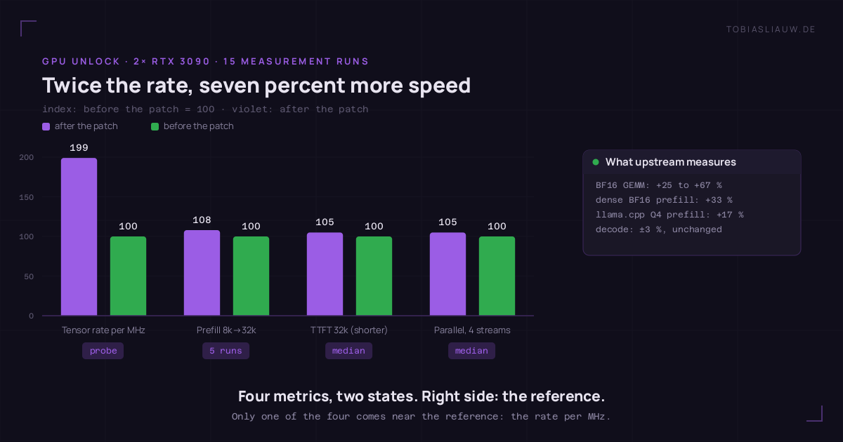
A kernel module promises to unlock the halved math rate of GeForce cards: twice as many instructions per clock cycle. After two days of measuring one thing is clear: the module does exactly what it says — measured 1.99 times the rate per clock cycle, across ten runs with less than 0.15 percent spread. My language model still only gets 7.5 percent faster. This post is an attempt to fit both numbers without bending either one.
The trigger was a kernel module called gpu-unlock that caused a stir in October, because it gives NVIDIA’s 3000-series cards a feature they technically have but aren’t allowed to use: the full issue rate of their tensor cores. This is not overclocking, not a tuning trick — it is a register the vendor sets differently per card family. I enabled it on my machine with two GeForce RTX 3090, because I need prefill throughput for my local models — and because after two days I can say: the hardware number is spectacular, the model number is disappointing, and both are true.
Everything measurable is attached below as a file: the full measurement log as CSV (eleven runs, before and after, with clock and power draw of the cards before every run, plus the hash of the output probe) and the raw text of my issue-rate probe (ten runs, both cards, including the calibration curve). If you want to check the claim „the module works”, the second file is all you need.
What the module actually does
On the same silicon NVIDIA uses different register values for its professional cards and for GeForce. The module writes two of those speed selectors — 0x88888888 for the full BF16 rate and 0x8 for another set of instructions — and it does so before the driver: it runs in the initramfs, in the early boot stage, writes the registers and then performs a bus reset of the card before the NVIDIA driver takes it over. That is why no patched driver is needed and no firmware is overwritten, and why the lock comes back on its own when you power the card off.
The effect in question is an issue rate: how many instructions the graphics card may push into its compute units per clock cycle. That is a property you can measure without any language model, and that is where my attempt got interesting. I had no CUDA toolkit on the machine, no PyTorch, no vendor math library. So I wrote the probe myself: 208 lines of C that talk to the card through the driver, and 175 lines of hand-written PTX that the driver compiles at run time. The upstream documentation describes the technique; my raw measurement text is attached.
What upstream measures — and what it doesn’t
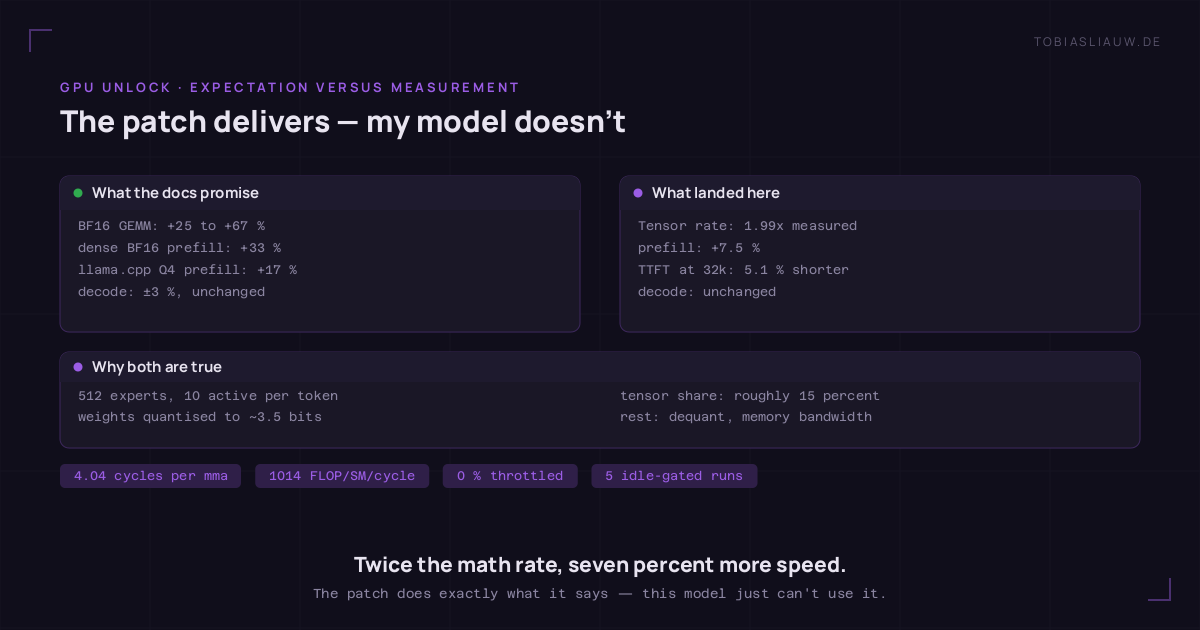
The project’s compatibility reports are a good source because they separate by workload. Read the headline table and you see „+25 to +80 percent” and think of language models. But the table measures something else.
| Source | Measured with | Result |
|---|---|---|
| project overview table | BF16 matrix multiplication, microbenchmark | RTX 3090: +25 to +67 % · RTX 3090 Ti: +68 to +80 % |
| report #25 | vLLM, 27-billion model in BF16, prefill | +33 % prefill, decode +1.2 % |
| report #158 | llama.cpp, Q4-quantised model, prefill at 100k context | +17 % prefill |
| report #152 | two RTX 3090, Proxmox/container, short prompt | time to first token 322 → 228 ms, decode −2.4 % |
| report #33 | one RTX 3090, rate per clock cycle measured | „about 2× FP16/BF16 per MHz” under a 350 W cap |
The project text itself says what this depends on: „The power limit matters a lot” — the lowest figure in the table comes from cards capped at 225 watts. My cards run at the usual 350 watts. That was my first guess, and it was wrong; more on that below.
My bar was set before the measurement
Before the first run I wrote down what counts as success, so I couldn’t bend the result afterwards. Agreed: prefill and time to first token +15 to +30 percent, decode unchanged to minus 3 percent, guardrail numbers unchanged. And the rule: if prefill stays below +15 percent, the parameter goes back out. That rule is uncomfortable because I want to keep the module — which is exactly why I wrote it down first.
Also agreed beforehand: the repeatability of the measurement has to be known, otherwise a seven percent gain is worthless. Two independent before-runs produced 2711.4 and 2709.1 tokens per second — the probe scatters by about 0.1 percent. That makes a seven percent difference measurable, and a 0.3 percent difference not.
The first run after the reboot was worthless
Enabling the parameter costs a reboot, and on a productive machine a reboot means 27 containers coming back up, a model fleet warming up, and requests from agents and containers that knew nothing about a benchmark. I ran the comparison measurement immediately after boot anyway — and it was rubbish: the cards were already busy at 1710 MHz and 107 watts when the measurement started, and the two repetitions of the decode run produced 42.8 and 52.0 tokens per second. Two repetitions of the same run may not differ by 20 percent, otherwise the run is not a measurement.
From that came a rule that saved the rest of the day: a measurement only starts when the cards are provably idle — clock at the idle value of 210 MHz and under 20 watts, measured twice in a row 15 seconds apart. The CSV documents this for every run: the columns karten_takt_vor_mhz and karten_leistung_vor_w. Two of the eleven runs carry the note „with foreign load” and are excluded from the medians.
The probe: rate per clock cycle instead of tokens per second
Tokens per second are a bad instrument for an issue rate, because memory bandwidth, queues, quantisation and batching all sit between the instruction and the result. So I measured directly what the module changes: per clock cycle. The probe starts one thread block per streaming multiprocessor, lets each warp issue four independent tensor core instructions per loop iteration and counts clock cycles with the block’s own clock counter. Because the result is stated per cycle, clock rate and power limit are divided out of the measurement — which makes it a good antidote to my wrong first guess.
| Quantity | GeForce stock (vendor spec) | full professional rate, same chip | measured, unlocked |
|---|---|---|---|
| work per thread block per clock cycle | 510 FLOP | 1093 FLOP | 1014 to 1015 FLOP |
| tensor core instruction, clock cycles per block | 8.00 | about 4.00 | 4.03 to 4.04 |
| projected to maximum clock, 82 blocks | 71.0 TF FP16 | 165 TF (RTX A6000) | 142.2 / 143.5 TF FP16 |
The number that actually convinced me is one line further down in the same file: the calibration curve. The same probe also measures ordinary floating point instructions on the CUDA cores, and their ceiling is fixed by the architecture: 128 units per block, two operations per instruction, so 256 FLOP per block per clock cycle. I measured 232.8 — 91 percent of what is possible, which is the expected issue gap with only four warps per block. Measured again: with 16 warps the same 128 units delivered 219 instead of 232 FLOP per cycle, because the warps then compete for the issue width. Had my probe shown 40 or 130 percent here, the tensor line would have been worthless.
And now the disappointing half: the production model
Five clean runs with idle cards, two measurement repetitions each, against three equally clean before-runs. Medians, because a single run is worth nothing here.
| Metric | before (median, n=3) | after (median, n=5) | difference |
|---|---|---|---|
| prefill, slope from 8k against 32k prompt | 2709.7 tokens/s | 2912.3 tokens/s | +7.5 % |
| time to first token, fresh 32k prompt | 12.98 s | 12.32 s | 5.1 % faster |
| time to first token, fresh 8k prompt | 3.91 s | 3.89 s | 0.5 % faster |
| parallel, four streams | 82.2 tokens/s | 86.5 tokens/s | +5.2 % |
| decode, 256 tokens including first token | 62.0 tokens/s | 69.3 tokens/s | no defensible value |
| output of a fixed test probe | SHA-256 864e30ed… |
SHA-256 864e30ed… |
bit-identical |
So I can claim nothing about decode. Twelve percent upwards would be too good to be true — decode is limited by memory bandwidth, every upstream report says so, and two of the runs measured it at the before level. Probably the serving program’s learned expert cache plays into it, but I cannot prove that here. I book decode as unchanged, which is the one place where I have to decide against my own measurement.
Why 7.5 percent and not 33 percent
Because my model does not do the work the patch was built for. The architecture is written in the metadata of the weight file, and I read it out instead of guessing:
| property | value from the weight file |
|---|---|
| shape | mixture of experts, 48 blocks, model width 2560 |
| experts | 512, of which 10 are active per token |
| width of one expert layer | 640 (plus one shared expert layer of 640) |
| attention heads | 24 query heads, 2 key/value heads |
| quantisation | IQ3_S, i.e. about 3.5 bits per weight |
| context length | 262,144 tokens |
| weight files | 55 GB plus 29 GB, plus a separate n-gram layer (3-token prediction) |
From that follows a calculation I can check, because it has to come out at the file size. One expert matrix consists of three weight matrices of size 2560 × 640, that is 4.9 million values. With 512 experts and 48 blocks that gives 120.8 billion expert weights, plus attention and router weights I land at about 123 billion values. At 3.5 bits per value that is 53.8 gigabytes — and the weight file is 55 gigabytes. So reading the architecture correctly.
And now the active side: 10 experts per token instead of 512, that is 2.36 billion expert values per token, plus attention, router and shared weights gives about 4.3 billion active values per token. One multiplication per value is two operations, so roughly 8.6 gigaflops per token. At the 2912 tokens per second I measured, that is 25 teraflops — 18 percent of what the unlocked card could do per second, but already 35 percent of what it could do in the factory state.
| route to the number | calculation | result |
|---|---|---|
| from the measurement (Amdahl) | +7.5 % total prefill at a doubled tensor rate | tensor share of prefill time: about 14 % |
| from the architecture (independent) | 25 TF achieved against 142 TF possible | utilisation of the tensor units: about 18 % |
The rest of the time goes where the patch cannot help: the weights first have to be turned back into numbers from 3.5 bits (dequantisation, which costs ordinary compute units), they have to be fetched from memory, the routing decision is made again per token, and the key/value caches are quantised to 8 bits on top. That is exactly why dense BF16 models see +33 percent and Q4 models +17 percent: the more real matrix work per token and the less conversion, the closer you get to the doubled rate.
My first guess was wrong: the power limit
I first thought: 350 watts instead of the 420 watts in the reference reports, hence the small gain. The upstream text suggests that, and the driver’s cumulative counters looked dramatic — at one point 2320 seconds of „software power cap” on one card. So I collected 1098 telemetry samples every two seconds during the measurement runs, logging the card’s throttle reason along with them.
| card | power in load samples (min / mean / max) | clock in load samples | throttled |
|---|---|---|---|
| first card | 16 / 166 / 203 watts | 1710–1980 MHz | 0 of 184 load samples |
| second card | 30 / 266 / 345 watts | 1665–1980 MHz | 0 of 325 load samples |
That makes the power-limit explanation refuted — and my issue-rate probe had already refuted it, because it measures per clock cycle and divides the limit out. A higher limit would only be a lever for dense BF16 work, not for my model.
What happened to the answers
The point I was most afraid of: a module that reaches into a graphics card’s computational entrails could change results. So I played a 44-probe behavioural sample — the same probes, the same categories as in an earlier run, so the comparison a week later was still the same comparison.
Result: all 44 probes played, no errors, the over-refusal of neutral technical questions is zero before and after the patch. Compliance dropped from 95.5 to 90.9 percent — that is a single difference out of 22 adversarial probes per run, and the number of probes the judge marked as disputed went from two to four. My fixed output probe returned the same SHA-256 hash in all eleven runs, and upstream reports also found outputs bit-identical.
I name the caveat myself: the judge runs on the same model family as the model under test, because an independent judge would need 55 gigabytes of weights. A single differing probe with four disputed ones is therefore no proof of a behaviour change — but also no proof of the opposite. What I can back up is the bit-identical fixed probe and the stability of the other 43 probes.
One more control story I nearly forgot
I wanted to re-measure the „dense” 27-billion model that the same fleet used to serve. My endpoint’s model list dutifully lists it. Except it is the same weights under a second name: the list shows four entries with identical alias fields, and a look at the running processes shows exactly one loaded model. So the „comparison” consisted of two runs against the same model, one of which fell into background load (time to first token: 18.11 seconds instead of 3.9) and one reached 2682 tokens per second prefill — 1 percent below the before value. A model list is not a statement about what is loaded; a process list is.
The real comparison against a dense model is therefore still outstanding, and it is the only sensible next test: but it needs a real measurement window, because 24 gigabytes of graphics memory are full, and for a before/after statement it also needs either another reboot with the parameter switched off, or one of the two cards that is not unlocked at boot.
Decision: keep it in
By my own pre-registered rule the parameter should come out, because 7.5 percent is below the 15 percent bar. I’m keeping it anyway, and I want to say transparently why — and what consequence I draw:
- The gain is real and tiny: +7.5 percent prefill, 5.1 percent shorter time to first token on long prompts, 5.2 percent more in parallel use, and it costs nothing but a parameter on the kernel command line.
- The costs are provably zero: decode unchanged, outputs bit-identical, no throttling, no firmware touched — the lock falls back by itself on power-off, and removing it is one parameter plus one reboot.
- The decision is a bet on the next model: a denser model, a model with more real matrix work per token, or a BF16 pass for image parts uses exactly the property that is now lying around unlocked. Broken down: I bought 7.5 percent today in order not to miss 30 percent when the right model arrives.
- The consequence I draw: I keep measuring at night. A timer writes the same measurement into the log every night at 1:20, so the decision about future parameters doesn’t rest on a single afternoon.
What I would do differently next time: don’t hang the bar on a percentage of the end result, but on two separate measurements — one close to the hardware that checks the patch, and one at the model that checks the benefit. The hardware one would have told me on day one that nothing is broken, and I wouldn’t have spent the afternoon chasing a power-limit relationship that didn’t exist. And the first run after the reboot would never have entered the evaluation at all.
Caveats
- One machine, two cards, one model. The issue-rate figure is a property of the chip and transfers as long as it is the same chip; the prefill gain hangs on the model and is measured for this model only.
- The active parameter count is computed, not measured. It comes from the metadata of the weight file (512 experts, 10 active, width 640, 48 blocks) and is supported by the file size — but I have no profiler that independently confirms the tensor share.
- The decode verdict is a choice, not a measurement. The five values are bimodal; I decided against an effect because the mechanism is missing and two values sit at the before level.
- The third measurement method has no before baseline. A second measuring program that builds its own prompts and hits no cache delivered 1775 / 1788 / 1780 tokens per second at 8k prompts (spread 0.7 percent) — but I never used it before the patch, so the numbers only serve as a continuity and scatter check.
- The judge is not independent. See above: same model family, no second judge available.
Artefacts and sources
Measurement log and raw probe text are linked: CSV measurement log (11 runs, 13 columns) · issue-rate probe, raw text (10 runs plus calibration) · graphics at full size: before/after (1200×630) and expectation against measurement (1200×630).
Sources: gpu-unlock, kernel module and compatibility reports (there the reports #25, #33, #152, #158 and the architecture write-up „How Ampere was unlocked”) · the quantised model whose metadata I computed from. On the guardrail test itself see the earlier posts „Same weights, two engines” and „One switch, 89 percentage points”, and on the machine „Three machines, one endpoint”.
Postscript, in case something changes: the timer keeps measuring every night, and the comparison against a dense model is still outstanding. If these numbers change I will update this post instead of writing a new one — the mistakes belong to it.
Update October 27: the prefill slope in this post (2709.7 → 2912.3 tokens/s) was counted in nominal prompt tokens, i.e. estimated from the character count, not in the tokens the model actually processed. In model tokens (usage.prompt_tokens) the unlocked rate is about 1980 tokens/s. Before and after were counted the same way, so the +7.5 percent ratio stands. The follow-up article measures in model tokens throughout: Four quant tiers, one afternoon: 84 to 128 tokens per second — and what the two bits cost.